Time series, a series of data points ordered in time. Pretty intuitive, isn’t it? Time series analysis helps in businesses in analyzing past data, predict trends, seasonality, and numerous other use cases. Some examples of time series analysis in our day to day lives include:
- Measuring weather
- Measuring number of taxi rides
- Stock prediction
In this blog, we will be dealing with stock market data and will be using Python 3, Pandas and Matplotlib.
Variation in Time Series Data
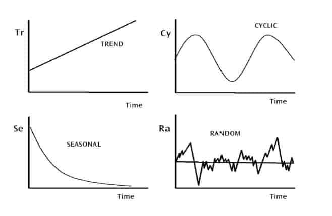
There are four types of variations in time series data.
- Trend Variation: moves up or down in a reasonably predictable pattern over a long period of time.
- Seasonality Variation: regular and periodic; repeats itself over a specific period, such as a day, week, month, season, etc.
- Cyclical Variation: corresponds with business or economic ‘boom-bust’ cycles, or is cyclical in some other form
- Random Variation: erratic or residual; doesn’t fall under any of the above three classifications.
Amazon Stock Data
To demonstrate the use of pandas for stock analysis, we will be using Amazon stock prices from 2013 to 2018. We’re pulling the data from Quandl, a company offering a Python API for sourcing a la carte market data. A CSV file of the data in this article can be downloaded from the article’s repository.
# Importing required modules
import pandas as pd
import numpy as np
import matplotlib.pyplot as plt

# Settings for pretty nice plots
plt.style.use('fivethirtyeight')
plt.show()

# Reading in the data
data = pd.read_csv('amazon_stock.csv')
A first look at Amazon’s stock Prices
# Inspecting the data
data.head()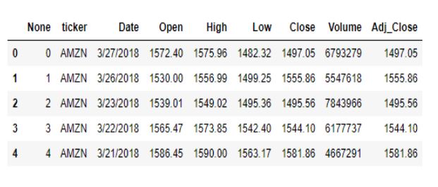
Let’s get rid of the first two columns as they don’t add any value to the dataset.
data.drop(columns=['None', 'ticker'], inplace=True)
data.head()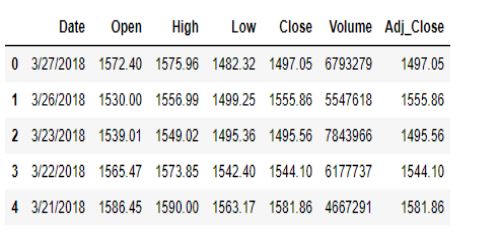
Let us now look at the datatypes of the various components.
data.info()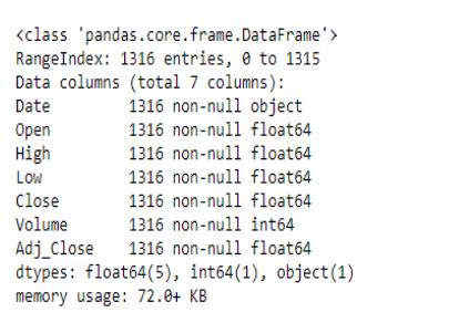
It appears that the Date column is being treated as a string rather than as dates. To fix this, we’ll use the pandas to_datetime() feature which converts the arguments to dates.
# Convert string to datetime64
data['Date'] = data['Date'].apply(pd.to_datetime)
data.info()
Lastly, we want to make sure that the Date column is the index column.
data.set_index('Date', inplace=True)
data.head()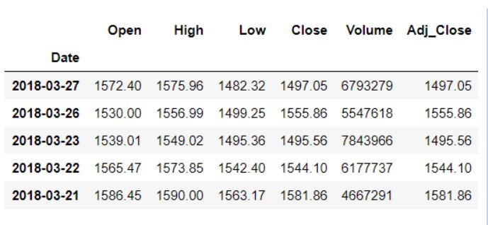
Now that our data has been converted into the desired format, let’s take a look at its columns for further analysis.
- The Open and Close columns indicate the opening and closing price of the stocks on a particular day.
- The High and Low columns provide the highest and the lowest price for the stock on a particular day, respectively.
- The Volume column tells us the total volume of stocks traded on a particular day.
The Adj_Close column represents the adjusted closing price, or the stock’s closing price on any given day of trading, amended to include any distributions and/or corporate actions occurring any time before the next day’s open. The adjusted closing price is often used when examining or performing a detailed analysis of historical returns.
data['Adj_Close'].plot(figsize=(16,8),title='Adjusted Closing Price')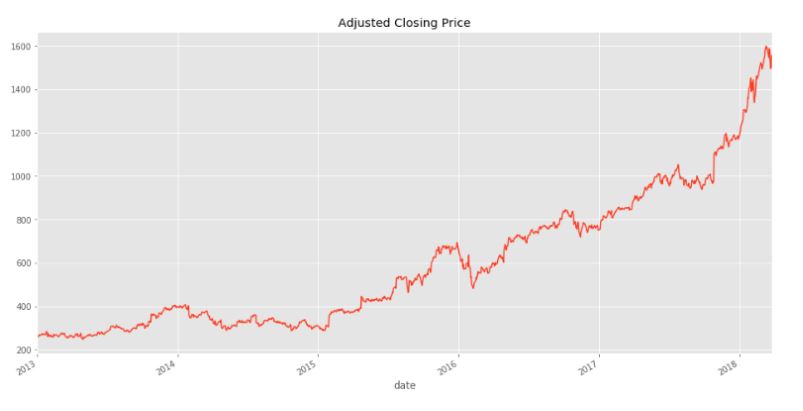
Interestingly, it appears that Amazon had a more or less steady increase in its stock price over the 2013-2018 window. We’ll now use pandas to analyze and manipulate this data to gain insights.
Pandas for Time Series Analysis
As pandas was developed in the context of financial modeling, it contains a comprehensive set of tools for working with dates, times, and time-indexed data. Let’s look at the main pandas data structures for working with time series data.
Manipulating datetime
Python’s basic tools for working with dates and times reside in the built-in datetime module. In pandas, a single point in time is represented as a pandas.Timestamp and we can use the datetime() function to create datetime objects from strings in a wide variety of date/time formats. datetimes are interchangeable with pandas.Timestamp.
from datetime import datetime
my_year = 2019
my_month = 4
my_day = 21
my_hour = 10
my_minute = 5
my_second = 30
We can now create a datetime object, and use it freely with pandas given the above attributes.
test_date = datetime(my_year, my_month, my_day)
test_date


# datetime.datetime(2019, 4, 21, 0, 0)
For the purposes of analyzing our particular data, we have selected only the day, month and year, but we could also include more details like hour, minute and second if necessary.
test_date = datetime(my_year, my_month, my_day, my_hour, my_minute, my_second)
print('The day is : ', test_date.day)
print('The hour is : ', test_date.hour)
print('The month is : ', test_date.month)

# Output

The day is :  21
The hour is :  10
The month is :  4
For our stock price dataset, the type of the index column is DatetimeIndex. We can use pandas to obtain the minimum and maximum dates in the data.
print(data.index.max())
print(data.index.min())

# Output

2018-03-27 00:00:00
2013-01-02 00:00:00
We can also calculate the latest date location and the earliest date index location as follows:
# Earliest date index location
data.index.argmin()
#Output
1315
# Latest date location
data.index.argmax()
#Output
0
Time resampling
Examining stock price data for every single day isn’t of much use to financial institutions, who are more interested in spotting market trends. To make it easier, we use a process called time resampling to aggregate data into a defined time period, such as by month or by quarter. Institutions can then see an overview of stock prices and make decisions according to these trends.
The pandas library has a resample() function which resamples such time series data. The resample method in pandas is similar to its groupbymethod as it is essentially grouping according to a certain time span. The resample() function looks like this:
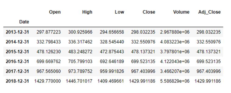
data.resample(rule = 'A').mean()To summarize:
data.resample()is used to resample the stock data.- The ‘A’ stands for year-end frequency, and denotes the offset values by which we want to resample the data.
mean()indicates that we want the average stock price during this period.
The output looks like this, with average stock data displayed for December 31st of each year
We can also use time sampling to plot charts for specific columns.
data['Adj_Close'].resample('A').mean().plot(kind='bar',figsize = (10,4))
plt.title('Yearly Mean Adj Close Price for Amazon')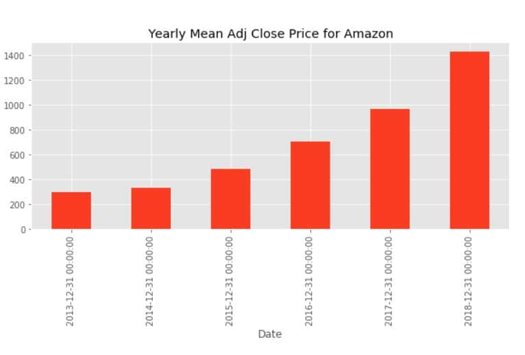
The above bar plot corresponds to Amazon’s average adjusted closing price at year-end for each year in our data set.
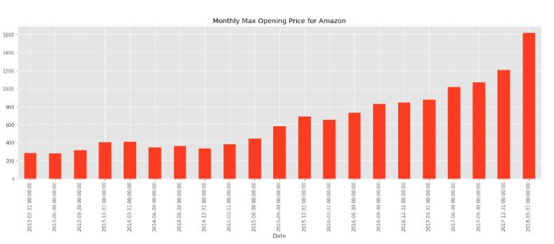
Similarly, monthly maximum opening price for each year can be found below.
Time shifting
Sometimes, we may need to shift or move the data forward or backwards in time. This shifting is done along a time index by the desired number of time-frequency increments.
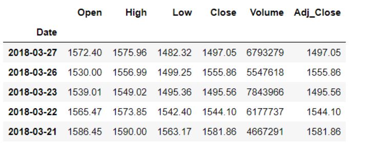
Here is the original dataset before any time shifts.
Forward Shifting
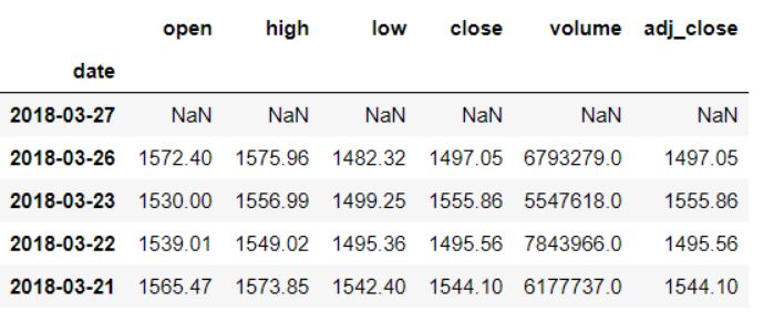
To shift our data forward, we will pass the desired number of periods (or increments) through the shift() function, which needs to be positive value in this case.
data.shift(1).head()Here we will move our data forward by one period or index, which means that all values which earlier corresponded to row N will now belong to row N+1. Here is the output:
Backwards shifting
To shift our data backwards, the number of periods (or increments) must be negative.
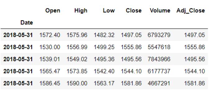
data.shift(-1).head()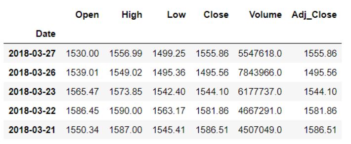
The opening amount corresponding to 2018–03–27 is now 1530, whereas originally it was 1572.40.
Shifting based off time string code
We can also use the offset from the offset table for time shifting. For that, we will use the pandas shift() function. We only need to pass in the periods and freq parameters. The period attribute defines the number of steps to be shifted, while the freq parameters denote the size of those steps.
Let’s say we want to shift the data three months forward:
data.tshift(periods=3, freq = 'M').head()We would get the following as an output:
Rolling windows
Time series data can be noisy due to high fluctuations in the market. As a result, it becomes difficult to gauge a trend or pattern in the data. Here is a visualization of the Amazon’s adjusted close price over the years where we can see such noise:
data['Adj_Close'].plot(figsize = (16,8))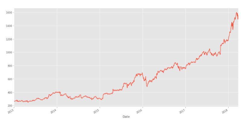
As we’re looking at daily data, there’s quite a bit of noise present. It would be nice if we could average this out by a week, which is where a rolling mean comes in. A rolling mean, or moving average, is a transformation method which helps average out noise from data. It works by simply splitting and aggregating the data into windows according to function, such as mean(), median(), count(), etc. For this example, we’ll use a rolling mean for 7 days.
data.rolling(7).mean().head(10)Here’s is the output:
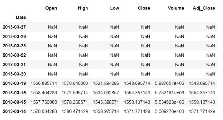
The first six values have all become blank as there wasn’t enough data to actually fill them when using a window of seven days.
So, what are the key benefits of calculating a moving average or using this rolling mean method? Our data becomes a lot less noisy and more reflective of the trend than the data itself. Let’s actually plot this out. First, we’ll plot the original data followed by the rolling data for 30 days.
data['Open'].plot()
data.rolling(window=30).mean()['Open'].plot(figsize=(16, 6))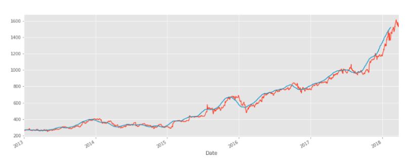
The orange line is the original open price data. The blue line represents the 30-day rolling window, and has less noise than the orange line. Something to keep in mind is that once we run this code, the first 29 days aren’t going to have the blue line because there wasn’t enough data to actually calculate that rolling mean.
Conclusion
Python’s pandas library is a powerful, comprehensive library with a wide variety of inbuilt functions for analyzing time series data. In this article, we saw how pandas can be used for wrangling and visualizing time series data.
We also performed tasks like time sampling, time shifting and rolling with stock data. These are usually the first steps in analyzing any time series data. Going forward, we could use this data to perform a basic financial analysis by calculating the daily percentage change in stocks to get an idea about the volatility of stock prices. Another way we could use this data would be to predict Amazon’s stock prices for the next few days by employing machine learning techniques. This would be especially helpful from the shareholder’s point of view.
Thanks for reading the article which originally appeared on Kite. I have written other posts related to software engineering and data science as well. You might want to check them out here. You can also subscribe to my blog to receive updates straight in your inbox.